Dynamic per-label thresholds for large-scale search query classification with Otsu’s method

Solving the “Which Score Is Good Enough?” Puzzle

The real-world problem

Arbitrary label search-query intent classifiers spit out a confidence score per label.

On clean demos you set one global cut-off say 0.50 and move on.

In production:

1. Some labels are rare and score conservatively.
2. Others are common and score generously.
3. A single global threshold either floods common labels onto everything or leaves rare labels starved.

Manual tuning per label quickly turns into a never-ending whack-a-mole, especially when the taxonomy is customized client-by-client (e.g., SaaS today, Gaming tomorrow).

Here’s an example:

Query: “used caravan shower cubicles for sale near me”

data = [

(“LOCAL”, 0.9697265625),

(“PRODUCT”, 0.83837890625),

(“CATEGORY”, 0.39892578125),

(“TRANSACTIONAL”, 0.09222412109375),

(“INFORMATIONAL”, 0.000947475433349609),

(“PROMO”, 0.00080108642578125),

(“BRANDED”, 0.00034332275390625),

(“SUPPORT”, 0.000284671783447266),

(“NAVIGATIONAL”, 0.000205039978027344),

]

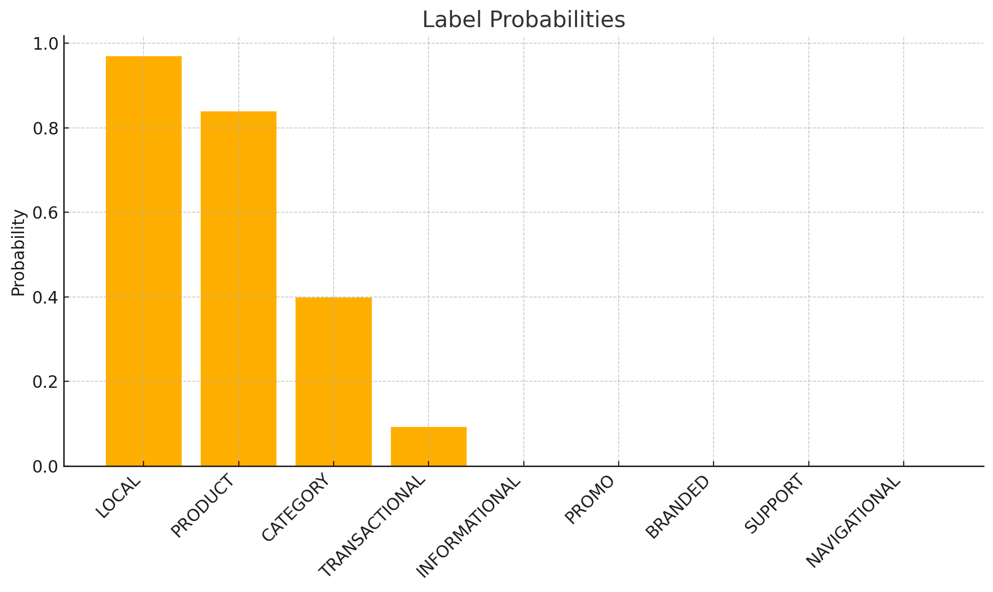
Well that’s easy you might say. It’s quite obvious we can set threshold to 0.4 and that sets LOCAL, PRODUCT and CATEGORY. We miss TRANSACTIONAL but otherwise keep the floodgates of irrelevant stuff out for other labels at that threshold value.

Right? Cool now let’s do another query.

Query: “square tents”

data = [

(“PRODUCT”, 0.84423828125),

(“CATEGORY”, 0.31689453125),

(“SUPPORT”, 0.00284576416015625),

(“TRANSACTIONAL”, 0.000590801239013672),

(“PROMO”, 0.000458240509033203),

(“BRANDED”, 0.00039362907409668),

(“INFORMATIONAL”, 0.000348806381225586),

(“LOCAL”, 0.000211477279663086),

(“NAVIGATIONAL”, 0.000198721885681152),

]

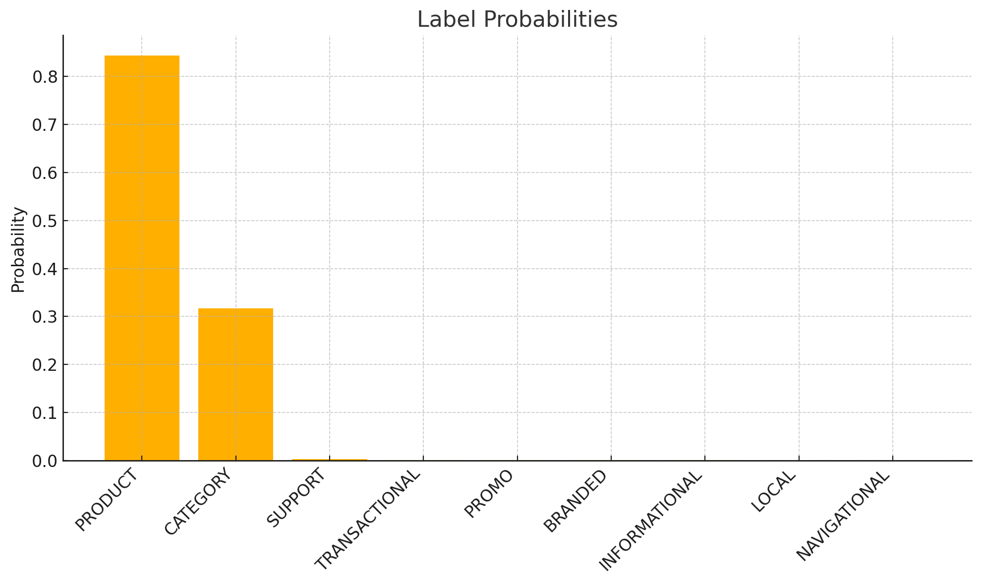
We’ll just use the same threshold. Right? Wrong! You now have to lower it to 0.3 to include the CATEGORY label. This is because all labels have different and inconsistent confidence thresholds.

Now imagine fiddling around like this with 100,000 queries?

No thanks.

Why Otsu helps

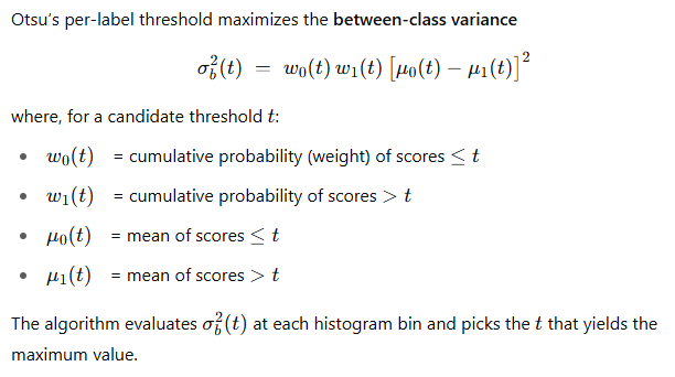
Otsu’s algorithm (1979) was built for image segmentation: find the gray-level that best separates foreground and background by maximizing between-class variance.

Translate to NLP:

1. Treat each label’s score distribution across all queries as a gray-scale histogram.
2. “Foreground” = confident positives; “background” = likely negatives.
3. The computed threshold adapts to each label’s own distribution; no hand tuning.

Picture your label-scores as a mountain range drawn by a histogram:

1. Left peak = all the “this label is probably false” scores
2. Right peak = all the “this label is probably true” scores
3. Valley (the dip) between the peaks = the score where those two crowds separate

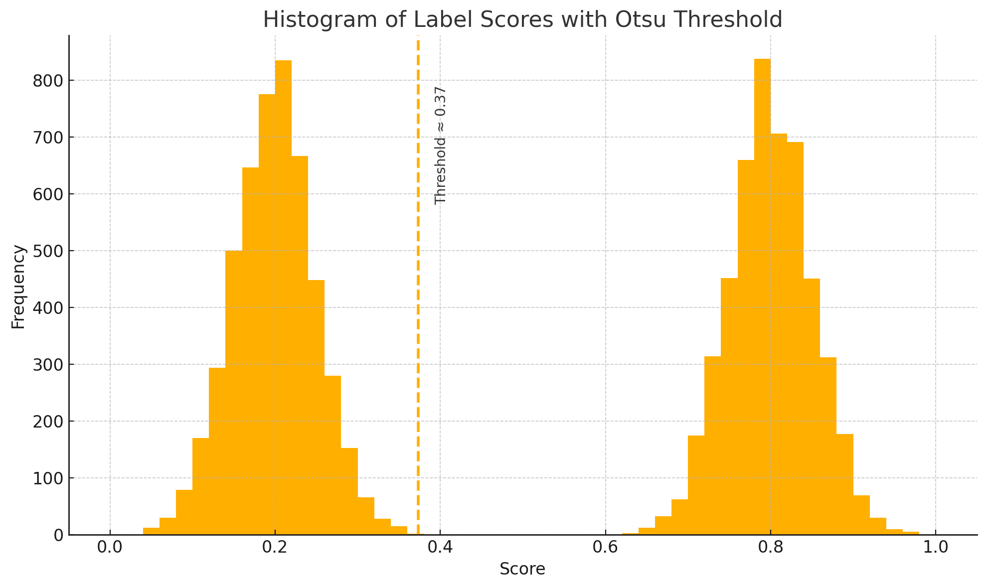Histogram illustrates two peaks (likely negatives on the left, positives on the right) with the dashed vertical line marking the Otsu-derived threshold at the lowest point between them.

Otsu simply slides a vertical ruler across that landscape, computes how well the left side and right side each cluster, and stops at the deepest point of the valley, the most natural dividing line. That valley score becomes the dynamic threshold for that label.

Implementation

def otsu_threshold(scores,bins=256): hist,edges=np.histogram(scores,bins=bins,range=(0.0,1.0)) centers=(edges[:-1]+edges[1:])/2 total=hist.sum(); sum_total=(hist*centers).sum() w_bg=sum_bg=best_var=best_t=0.0 for i in range(bins): w_bg+=hist[i] if w_bg==0 or w_bg==total: continue w_fg=total-w_bg; sum_bg+=hist[i]*centers[i] mean_bg=sum_bg/w_bg; mean_fg=(sum_total-sum_bg)/w_fg var_between=w_bg*w_fg*(mean_bg-mean_fg)**2 if var_between>best_var: best_var,var_between=var_between,var_between; best_t=centers[i] return best_t
def apply_otsu_tagging(set_id,bins=256): conn=get_db_connection() df=pd.read_sql("SELECT query_id,label,score FROM classification_scores WHERE set_id = ?",conn,params=(set_id,)) thresholds={lbl:otsu_threshold(grp['score'].values,bins) for lbl,grp in df.groupby('label')} df['threshold']=df['label'].map(thresholds) keep=df[df['score']>=df['threshold']] tag_map=dict(pd.read_sql("SELECT label,tag_id FROM uqc_label_tags WHERE set_id = ?",conn,params=(set_id,)).values) to_insert=keep[['query_id','label']].drop_duplicates() rows=[(int(r.query_id),int(tag_map[r.label])) for r in to_insert.itertuples() if r.label in tag_map] cur=conn.cursor() cur.executemany("INSERT OR IGNORE INTO query_tags (query_id,tag_id) VALUES (?,?)",rows) conn.commit(); conn.close()

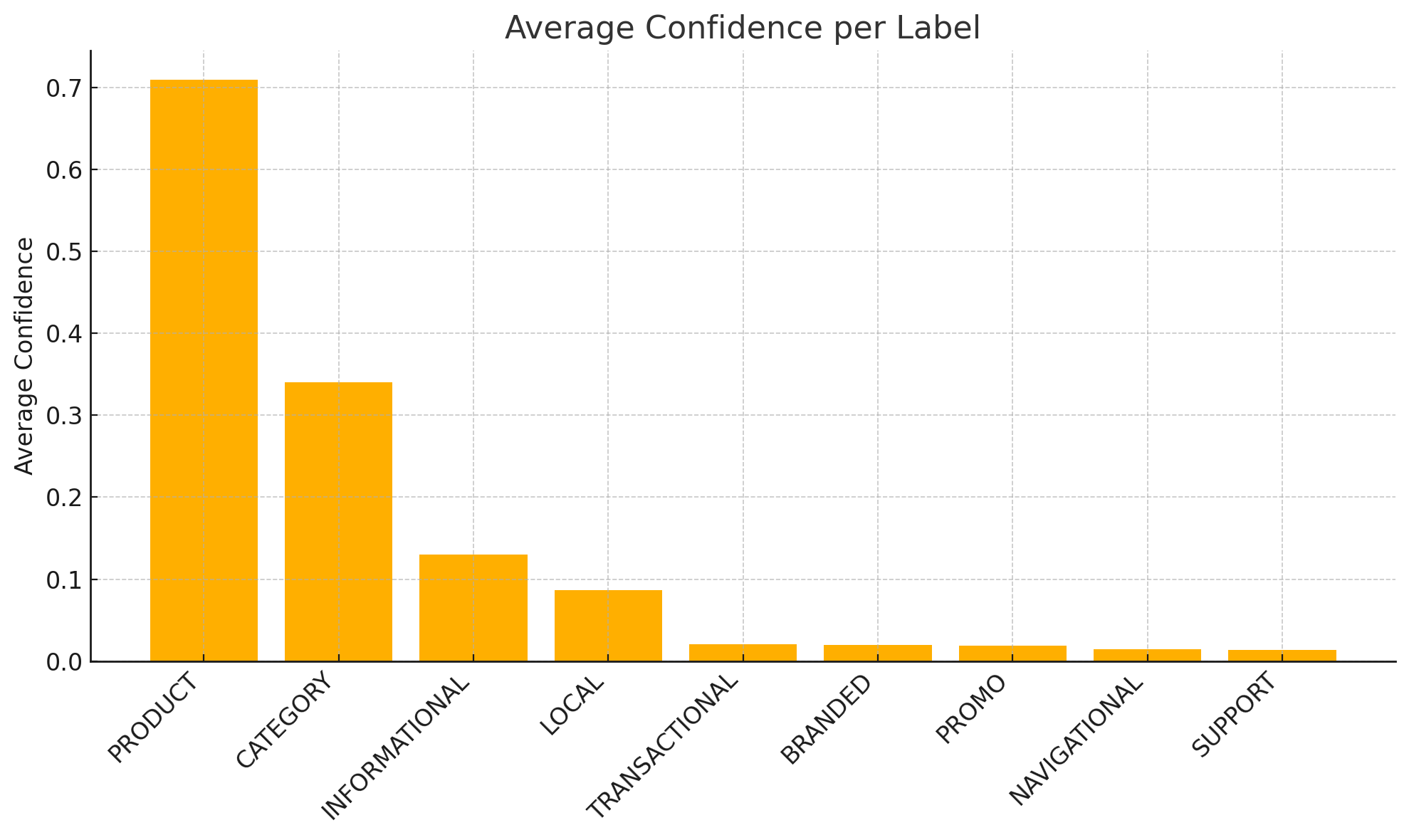
scores are that label’s confidences across the full corpus.

Recalculate thresholds every time you re-score so they drift with model upgrades or seasonal traffic changes.

Edge cases and the fallback rule

1. Bi-modal distributions Otsu excels.
2. Mono-tonic everything low Otsu returns a tiny threshold; you risk false positives.
3. Fix: keep a global floor (e.g., 0.25) below which nothing is labeled.
4. No label survives about 12 % in our first run.
5. We added: if a query gets zero labels, assign the single highest-scoring one only if its score > 0; if two labels tie at that max, keep both.
6. This fills holes without spraying labels everywhere.

Results

RunGlobal cut-offOtsu per-labelFallback% queries with ≥1 labelAvg labels/queryBaseline0.50

88 %1.9Static 0.350.35

99 %3.7 noisyOtsu + floor 0.250.25✓
96 %2.1Otsu + floor 0.25 + fallback0.25✓✓100 %2.3

Noise stayed manageable while eliminating unlabeled rows.

Takeaways

1. Per-label score landscapes differ wildly; one threshold cannot rule them all.
2. Otsu is a zero-tuning, data-driven way to derive label-specific cut-offs.
3. Guardrails global floor plus intelligent fallback curb the method’s rare failure modes.
4. The approach scales effortlessly to any arbitrary taxonomy drop in new labels, rerun, done.

Dynamic thresholding solved without manual babysitting.